Bayesian Mixture models: A Success Story for MCMC Methods
Stanley Sawyer
Abstract:
Mixture models --- in which a population is modeled as a small number of
discrete subpopulations, each with their own parameters, turn out to work
unexpectedly well in a Bayesian framework. (This from a confirmed,
lifelong non-Bayesian.)
The goal with mixture models is to estimate the relative sizes of the subpopulations, get some information about which subjects belongs to what subpopulations, and estimate the parameters for each subpopulation. After giving a brief introduction to MCMC, we will speculate as to why MCMC methods work so well on some mixture models. If there is time, we will also discuss an application in which these methods were helpful as part of a larger project.
Transparencies for Talk
(PDF format)
(Mixture models, some genetics and probability for an ongoing
application, using MCMC to estimate parameters)
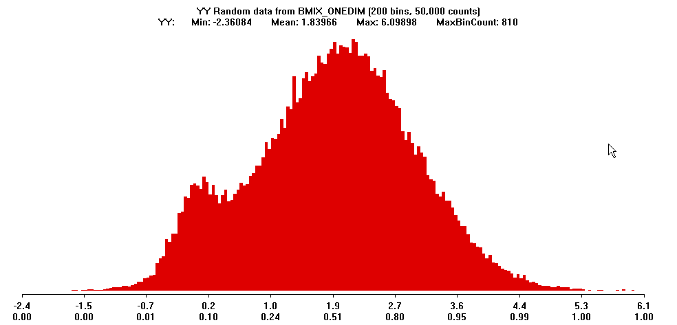
Two examples of data from mixtures of normal subpopulations:
Example 1: A population with an obvious distinguished subsample
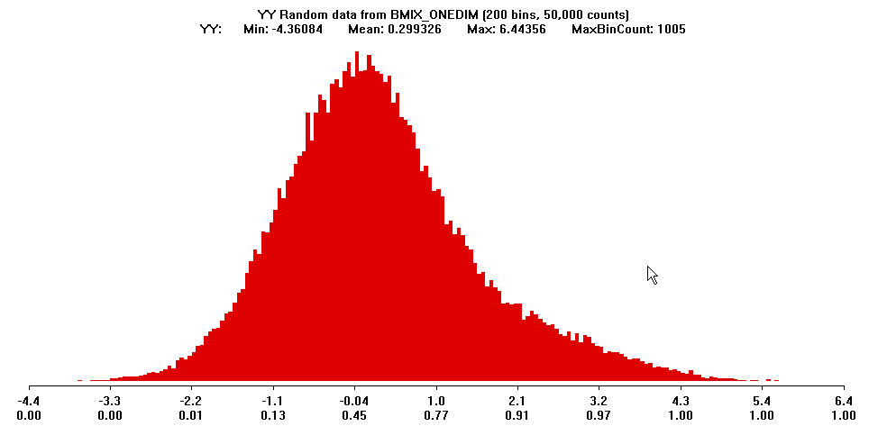
Example 2: A heavy-tailed unimodal distribution that is actually a
mixture of two normal subpopulations
A natural MCMC chain for a Bayesian normal mixture model assuming
exactly two components converges in these examples (but with some difficulty)
and estimates parameters for the two components:
Example 1:
An Application in Genetics:
The Main Parameters:
Mugamma:
The overall mean of selection coefficients over 73 genetic loci
Wsigma:
The standard deviation of selection coefficients of new mutants within loci
Bsigma:
The standard deviation of locus means across loci
The following are plots generated from 5000 equally-spaced values from two run of a high-dimensional Markov Chain with 21,000,000 or 5,500,000 iterations.
The three main parameters are correlated and have a TRIMODAL distribution in the full run:
The full run goes back and forth between modes (1,2) and mode 3:
An informative prior can be used to block out the third mode:
Now there are only two mildly overlapping modes, but the distribution is
obvious bimodal:
Return to Stanley Sawyer non-course handout home page
Last modified November 1, 2006